TD 1 - Clustering via Mode Seeking
The goal of this lab session is to implement the graph-based
hill-climbing algorithm of Koontz et al., together with its variant ToMATo based on topological persistence. Both were presented during the lecture.
Graph-based hill-climbing
Class Point
Create a class Point with the following attributes and methods:
- an instance attribute coords (a tuple), to store the coordinates of the point,
- a method sqrt_distance(point_a, point_b), which computes the squared Euclidean distance between two points,
- a method __str__ for pretty printing on the console... :-)
Class HillClimbing
Create now a class HillClimbing with the following attributes:
- cloud, a list to store the data points,
- neighbors, a list to store the indices of the neighbors of each data point in the neighborhood graph (one list per point),
- density, a list to store the density values at the data points (one value per point),
- parent, a list to store the parent of each point in its cluster tree,
- label, a list to store the cluster label of each point.
Add the following methods:
- read_data(filename), to read the data points from a file and store it in cloud,
- compute_neighbors(k), to compute and store the k-NN graph of the data points. For this you can apply a naive strategy and compute all the pairwise distances (watch out that a point does not belong to its k-NN set).
- compute_density(k), to compute and store a density estimate at every data point. For this you can use the so-called distance to measure, defined as the average of the squared distances of the data point to its k nearest neighbors. The value of the density estimate is then the inverse of the square root of that quantity:
\( f(p) = \frac{1}{\sqrt{\tfrac{1}{k}\sum\limits_{q \in k\text{-NN}(p)} \lvert p-q \rvert^2}} \)
- compute_forest(k), to connect each data point to its parent, which is its neighbor in the k-NN graph with highest density value among the ones with strictly higher density (if they exist) or itself (otherwise).
- compute_labels(), to extract the clusters' labels from the array of parents. Note that the labels do not have to be contiguous nor to start at 0. Hence, you can simply take the index of the root of the tree for each cluster.
Tests
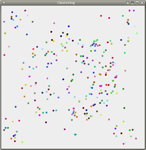
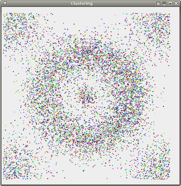
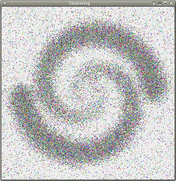
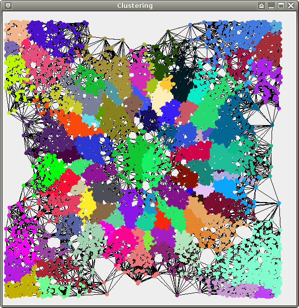
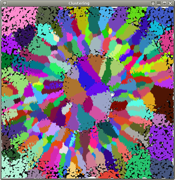
We provide 3 data sets for your
tests: test.xy (256
points), crater.xy (same distribution,
10000 points), and spirals.xy (about
70000 points). All 3 of them are 2-dimensional and therefore easy to
visualize, which should make your life easier for debugging. Here are
some pretty pictures (from left to right: test, crater, spirals):
Similar pictures can be captured by the Python script: clustering_window.py, which you can download and put together with the other source files. To use it, simply add the following instruction:
cluster(cloud, labels, neighbors, k)
where each parameter corresponds to a fields of your class HillClimbing, except for k which you must choose smaller than the number of neighbors in your neighborhood graph.
We recommend you test your code on the data set test first, to have fast runs and easy debugging. Then you can proceed with crater (takes a few dozens of seconds to handle on a decent machine), and then finally spirals (takes about half an hour). Try the following sets of parameters:
// parameters for test.xy
kDensity = 10;
kGraph = 5;

// parameters for crater.xy
kDensity = 50;
kGraph = 15;

// parameters for spirals.xy
kDensity = 100;
kGraph = 30;
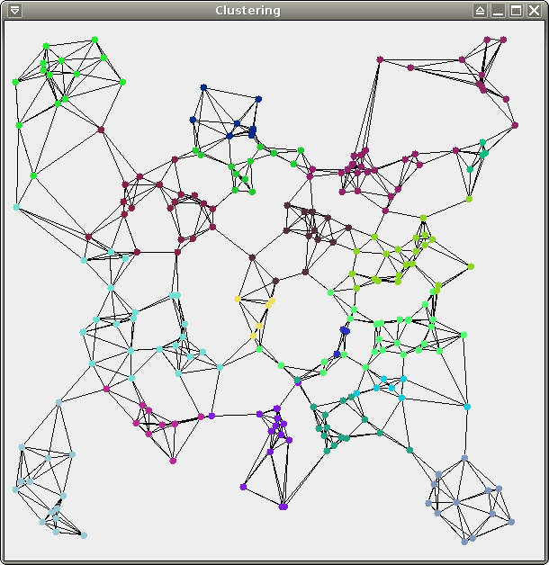
You should obtain the following results (19 clusters for test, 92 clusters for crater, 273 clusters for spirals):
ToMATo
Add the following method to your class HillClimbing:
- compute_persistence(k), which sorts the data points by decreasing estimated density values, then computes the 0-dimensional persistence of the superlevel sets of the density estimator via a union-find on the k-NN graph. At this stage you do not have to implement a full-fledged union-find, just use the trees stored in the field parent to do the merges. Whenever a cluster C is to be merged into another cluster C', simply hang the root of the tree of C to the root of the tree of C'.
Modify now your method compute_persistence as follows:
- compute_persistence(k, tau), which merges only the clusters whose corresponding density peaks have prominence less than tau.
You can test your code on the previous data sets using the following sets of parameters:
// parameters for test.xy
String filename = "test.xy";
kDensity = 10;
kGraph = 5;
tau = 0.35;

// parameters for crater.xy
String filename = "crater.xy";
kDensity = 50;
kGraph = 15;
tau = 2;

// parameters for spirals.xy
kDensity = 100;
kGraph = 30;
tau = 0.03;
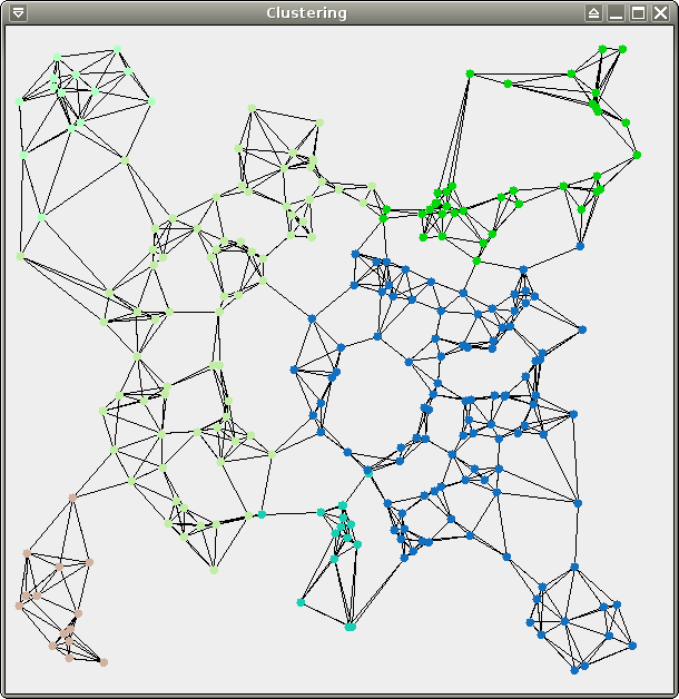
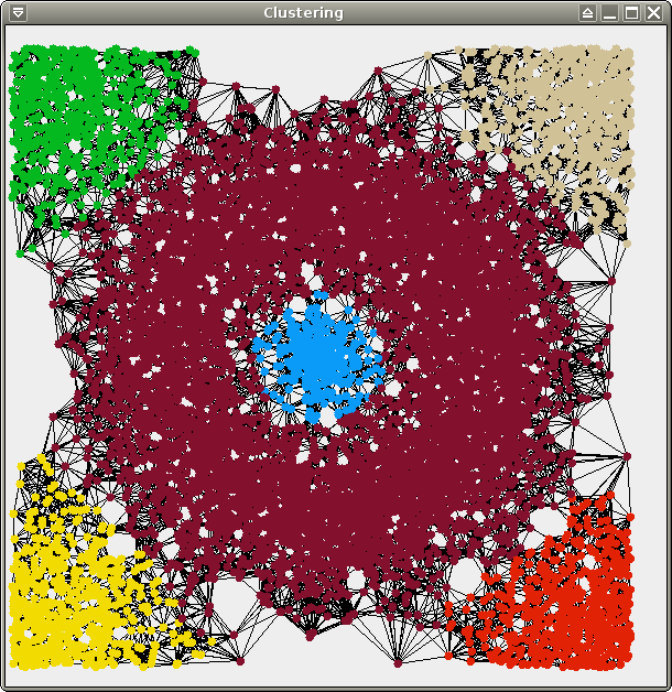
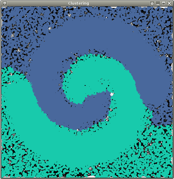
You should obtain the following results (6 clusters for test and crater, 2 clusters for spirals):
You can also make your method compute_persistence output the
sorted list of the prominences of the various density peaks. If you
plot this sequence of prominences, then you will see the `prominence
gap' corresponding to the aforementioned numbers of clusters.
Optimizations
The pacing phase of the pipeline is clearly the computation of the
neighborhood graph. It takes quadratic time in the input point,
regardless of the sparsity of the resulting graph. To optimize this phase you have several options:
- Implement your own data structure for efficient proximity queries, kd-tree for instance. For this you can refer to Section 1 of the following TD from INF562 for building and queryig a kd-tree, and if you have more time you can even do the whole TD which is about Mean-Shift, the other mode-seeking algorithm mentioned in today's lecture. :-)
- If your data points lie in 2D or 3D, then you can build
their Delaunay triangulation. Then, the k-NN of each data point are found among its neighbors, their own neighbors, etc. within the triangulation, hence by a simple graph traversal. For this you can refer to the session on Delaunay triangulations in the course INF562.
- You can also convert your code to C++ and use one of the existing libraries for NN search, such as ANN (which is based on a variant of the kd-trees and is extremely efficient in low and medium dimensions). This is probably the best option for optimizing this part of you code.
The other part of the code that can be optimized is the persistence
calculation. Until now we merely used the field parent to
store the trees of the clusters during the merging process. The
entailed complexity may be up to quadratic, although this rarely
happens (if at all) in practice. Now you can implement a
full-fledged union-find
data structure, with intelligent merges and path compression. This should keep the persistence calculation to a near-linear complexity.
Here is our solution in Python (HillClimbing.zip) and in Java (Point.java and HillClimbing.java) without optimizations.