TD 4 - Topological Persistence

Guidelines:

• you can work in groups of 2 to 3 people (1 submission per group only, but the report should mention the names of all the group members)
• submit your work on Moodle [submission link] as a single archive file by Tursday Oct. 24th 11:59pm CEST at the latest (no late submissions!)
• you can use whichever language you want (preferably Java, C/C++, or Python), including its standard library, but no external libraries that provide sparse matrix algebra (e.g. Boost, LAPACK, Eigen, or NumPy)
• you should submit your code (with comments), your filtration files, and a short report (a few pages) detailing the structure of the code and how to compile/run it, a short analysis of its complexity, and the answers to the questions asked in the TD.
• for your information, our solution code (in C++) has the following running times on the filtrations of Section 3.2 (on a standard laptop):
  • filtration A: 13 seconds
  • filtration B: 1.6 seconds
  • filtration C: 3 seconds
  • filtration D: 85 seconds
  
  

  The goal of this lab session is to implement an algorithm to compute persistent homology with coefficients in the field Z/2Z (also denoted Z₂ for short), and to test it on various filtrations.

  0. Input Filtrations

  We provide code to read filtrations. You can download it either in C++ or in Java. You can otherwise reproduce it in any other language of your choice.

  This code assumes that the filtration is given in an ASCII file with the following format, where each line represents a simplex sigma and is of the form:
  
  f(sigma) dim(sigma) v_0 ... v_{dim(sigma)}
  
  where:

  • f(sigma) is the function value of sigma (its "time of appearance" in the filtration),
  • dim(sigma) is the dimension of sigma,
  • v_0 ... v_{dim(sigma)} are the IDs (integers) of the vertices of sigma.

  For instance, 0.125 2 2 6 4 denotes a 2-simplex (triangle) that appears in the filtration at time 0.125 and whose vertices have IDs 2, 6 and 4. Warning: the function values provided in the file must be compatible with the underlying simplicial complex (function values of simplices must be at least as large as the ones of their faces). Nevertheless, the vertex IDs are arbitrary integers and may not start at 0 nor be continuous.

  The code produces a vector of simplices F, each simplex being described as a structure with fields val (float), dim (integer) and vert (the sorted set of the vertex IDs of the simplex). Warning: the order of the simplices in F may not be the one of the filtration.

  In order to help you debug your code during the course of the TD, here is a small sample filtration:

  6.0 2 1 7 4
  3.0 0 7
  5.0 1 4 1
  4.0 1 4 7
  2.0 1 4 2
  2.0 1 1 2
  1.0 0 2
  1.0 0 4
  4.0 1 7 1
  1.0 0 1
  

  The code you will be implementing should produce the following output barcode on this filtration:

  0 1.0 inf
  0 1.0 2.0
  0 1.0 2.0
  0 3.0 4.0
  1 4.0 inf
  1 5.0 6.0
  

  Do not hesitate to generate other toy examples to debug your code!

  1. Boundary Matrix

  Q1. Compute the boundary matrix B of the filtration from the vector of simplices F. Recall that we are working with coefficients in Z₂, so B is a binary matrix. You can choose either a dense or a sparse representation. Note that a dense representation is easier to work with, while a sparse representation scales up much better in terms of memory usage. A possible strategy is to do the TD using a dense representation, then to modify your code to use a sparse representation when you feel the need to be more space efficient, which will most probably happen in the final part of the TD.

  Note: before building the boundary matrix you need to sort F according to the filtration order.
  
  

  2. Reduction

  Q2. Implement the reduction algorithm for your representation of the boundary matrix. Evaluate its complexity.

  Q3. Reduce the complexity of the reduction to O(m^3) in the worst case, and to O(m) in cases where the matrix remains sparse throughout, where m is the number of simplices in the filtration. Argue that your code does have the desired worst-case and best-case complexities.

  Q4. Write a function that outputs the barcode from the reduced boundary matrix in a file. The format must be the following one: 1 line per interval, containing 3 numbers: the dimension of the homological feature associated with the interval, the left endpoint of the interval (which is the filtration value associated with the simplex that created the homological feature), the right endpoint (which is the filtration value associated with the simplex that killed the homological feature), separated by white spaces. For instance, interval [b,d) in dimension k is written k b d.

  3. Experiments

  3.1 Classical spaces

  Q5. Compute (by hand or with a generating code) filtrations for the d-sphere and the d-ball (d <= 10), the Moebius band, the torus, the Klein bottle and the projective plane. These last 4 spaces are each obtained from the square by gluing opposite edges as illustrated in the images below. Make sure that your filtrations are simplicial. Important: you should provide a drawing of your filtrations to ease the grading. You can choose whichever filtration values you want, provided that they satisfy the property that each simplex appears no sooner than its faces.

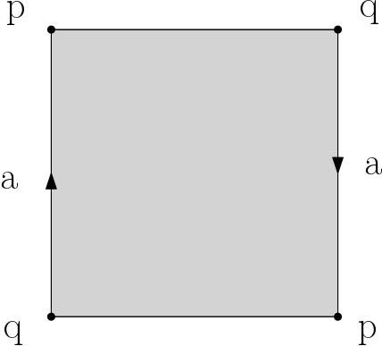  Moebius band

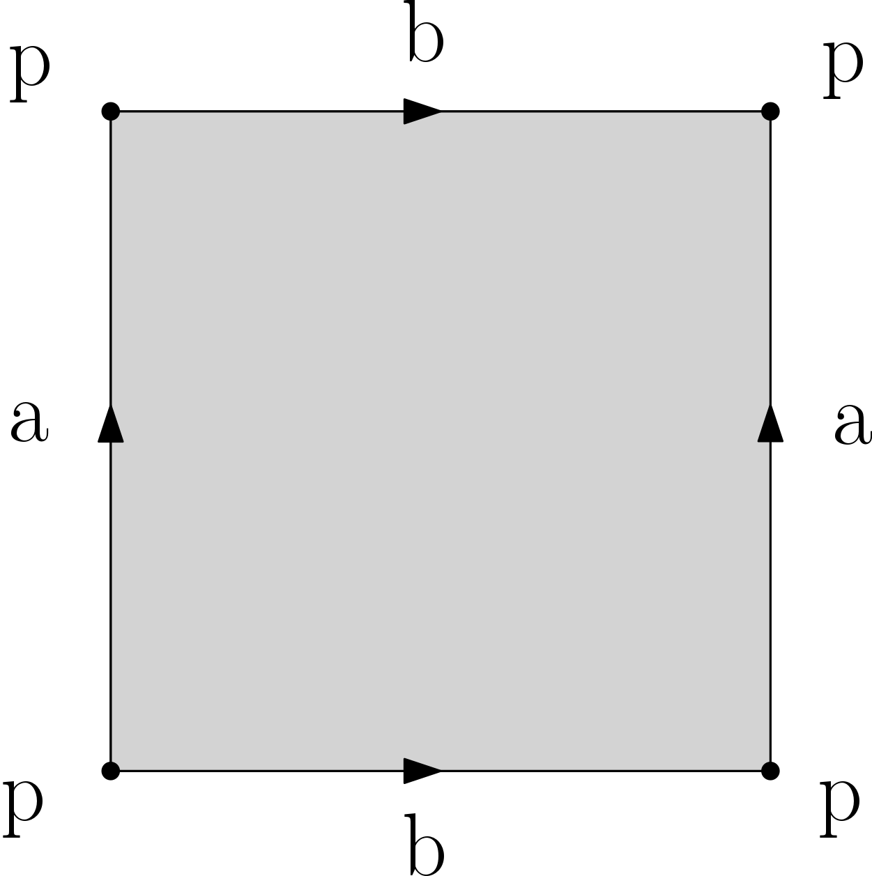  Torus

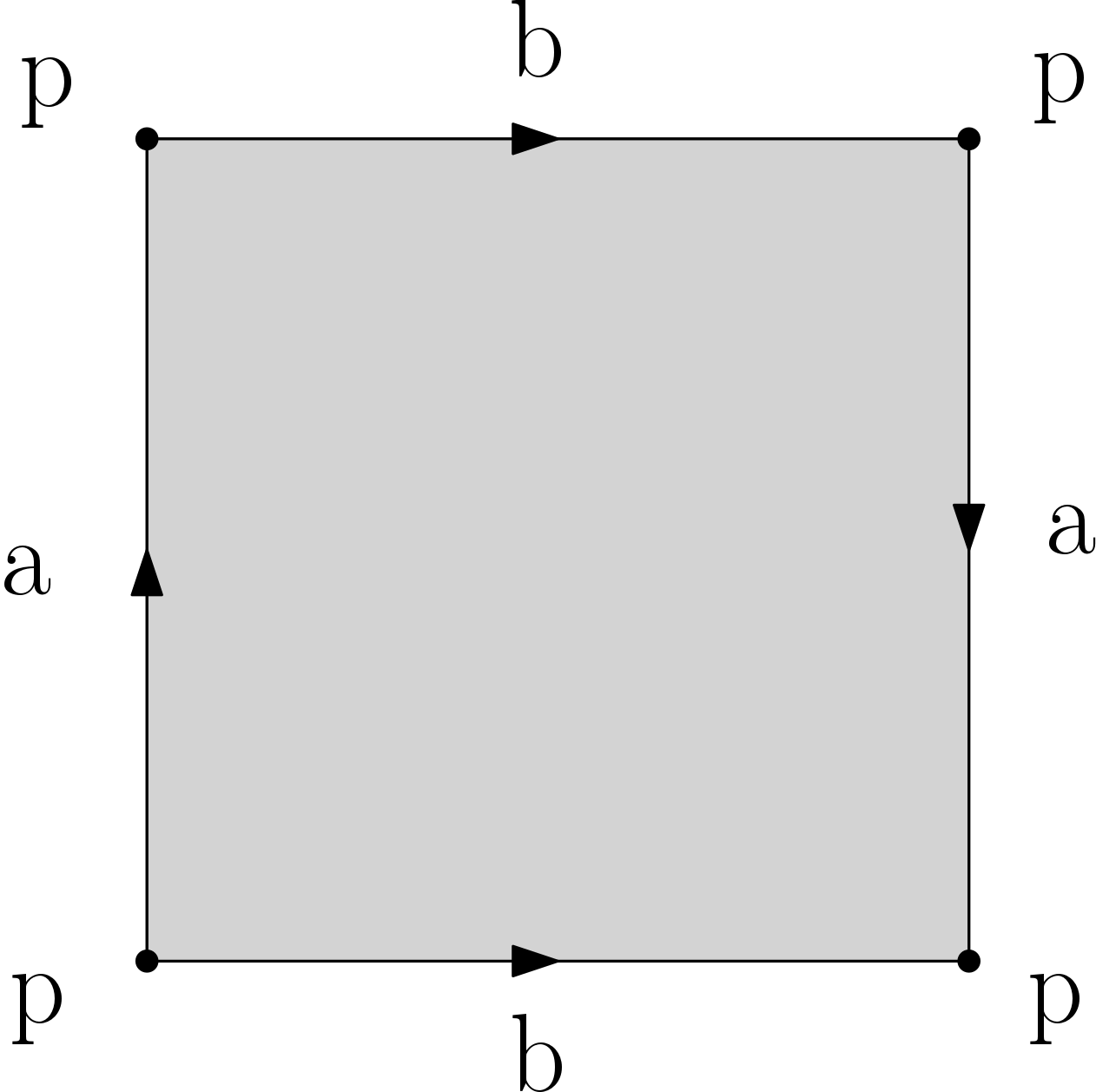  Klein bottle

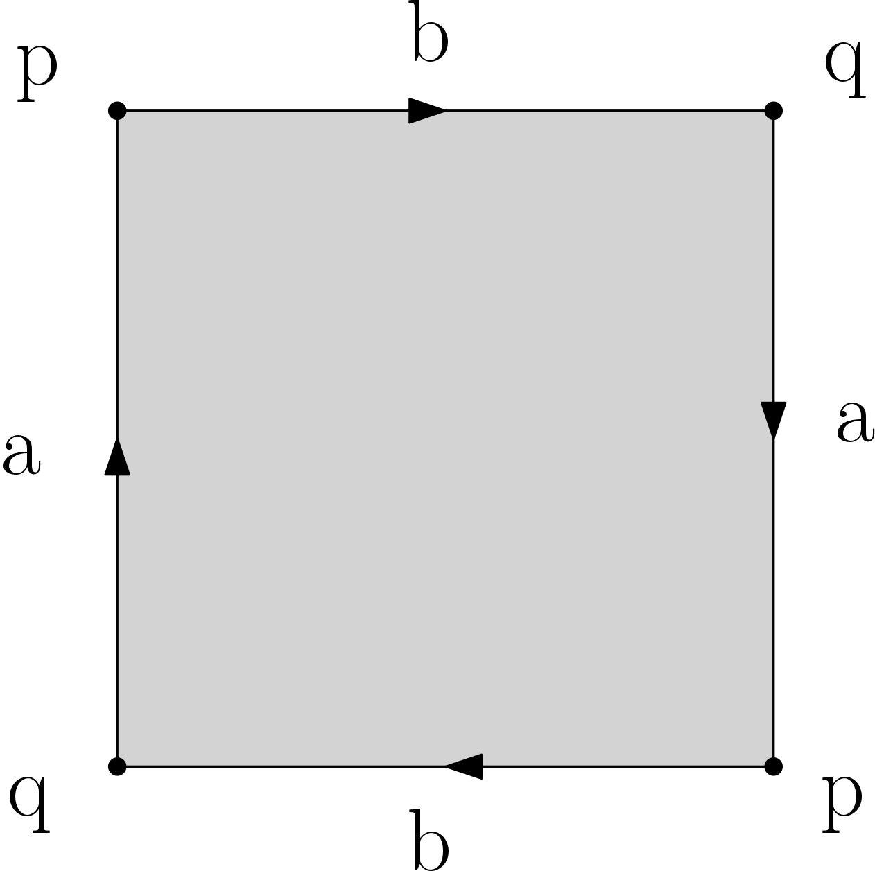  Projective plane

  Q6. Compute the barcodes of your filtrations using your code, and check the validity of your results against what is known about the homology of the underlying spaces.

  3.2 Simulated data

  We provide filtrations generated from simulated data. More precisely, for each filtration we started from a point cloud in some Euclidean space, then we built a simplicial filtration that is topologically equivalent to the offsets (unions of balls) filtration.

  Q7. Report the timings of your code on these filtrations. Compare them against your theoretical evaluation of its complexity.

  Q8. Can you infer the topological structure of the spaces underlying the data? To help you in this task, we show pictures of the barcodes obtained on these filtrations below (click on an image to see it at full resolution). Note that the barcodes A and D are represented on a logarithmic scale, and that for barcode B we have removed all the bars of length less than 0.05 to improve the visibility of the most important bars.

  filtration A: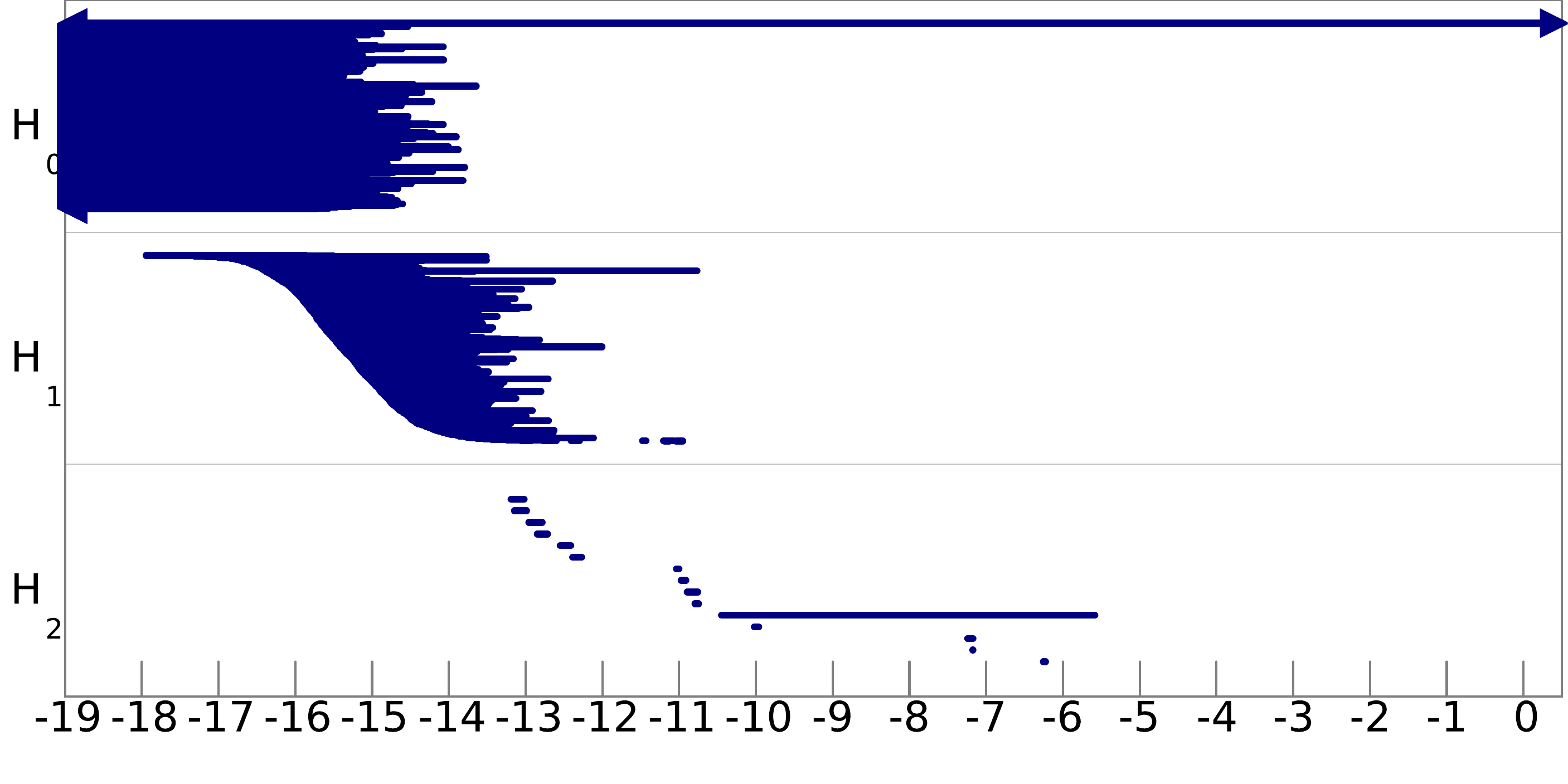	filtration B: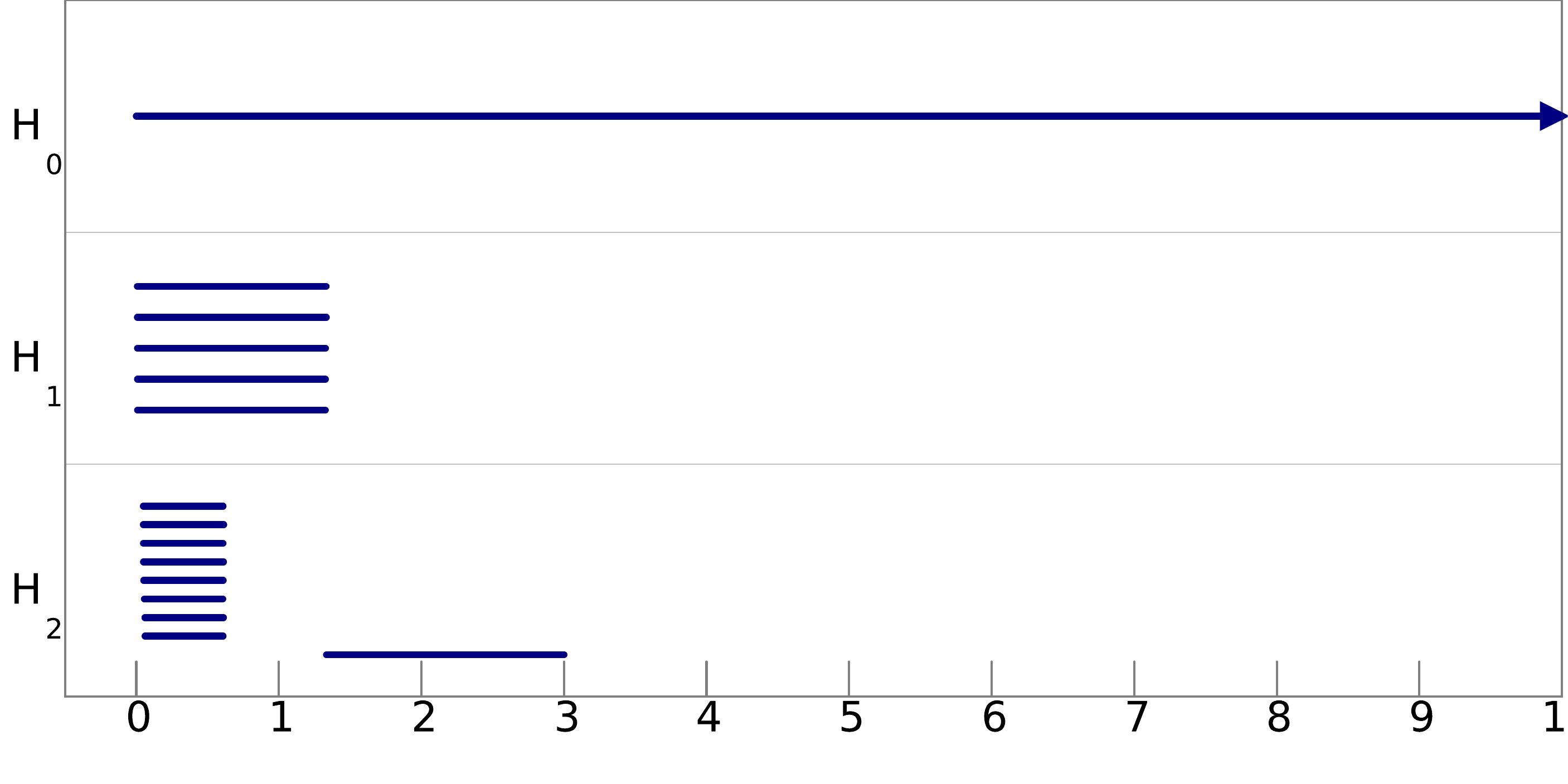
  filtration C: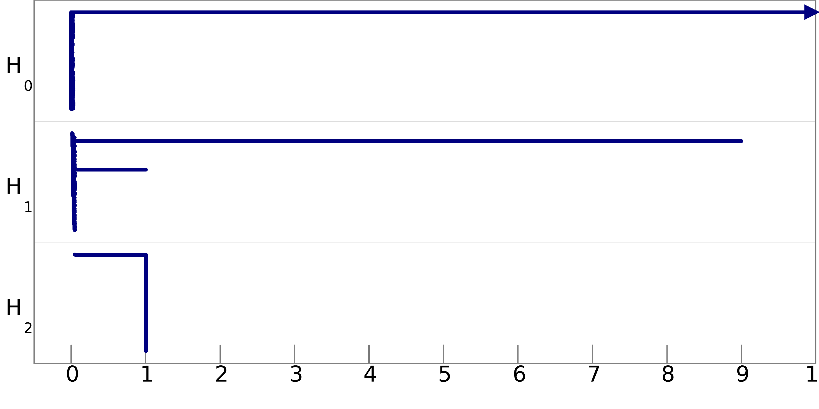	filtration D: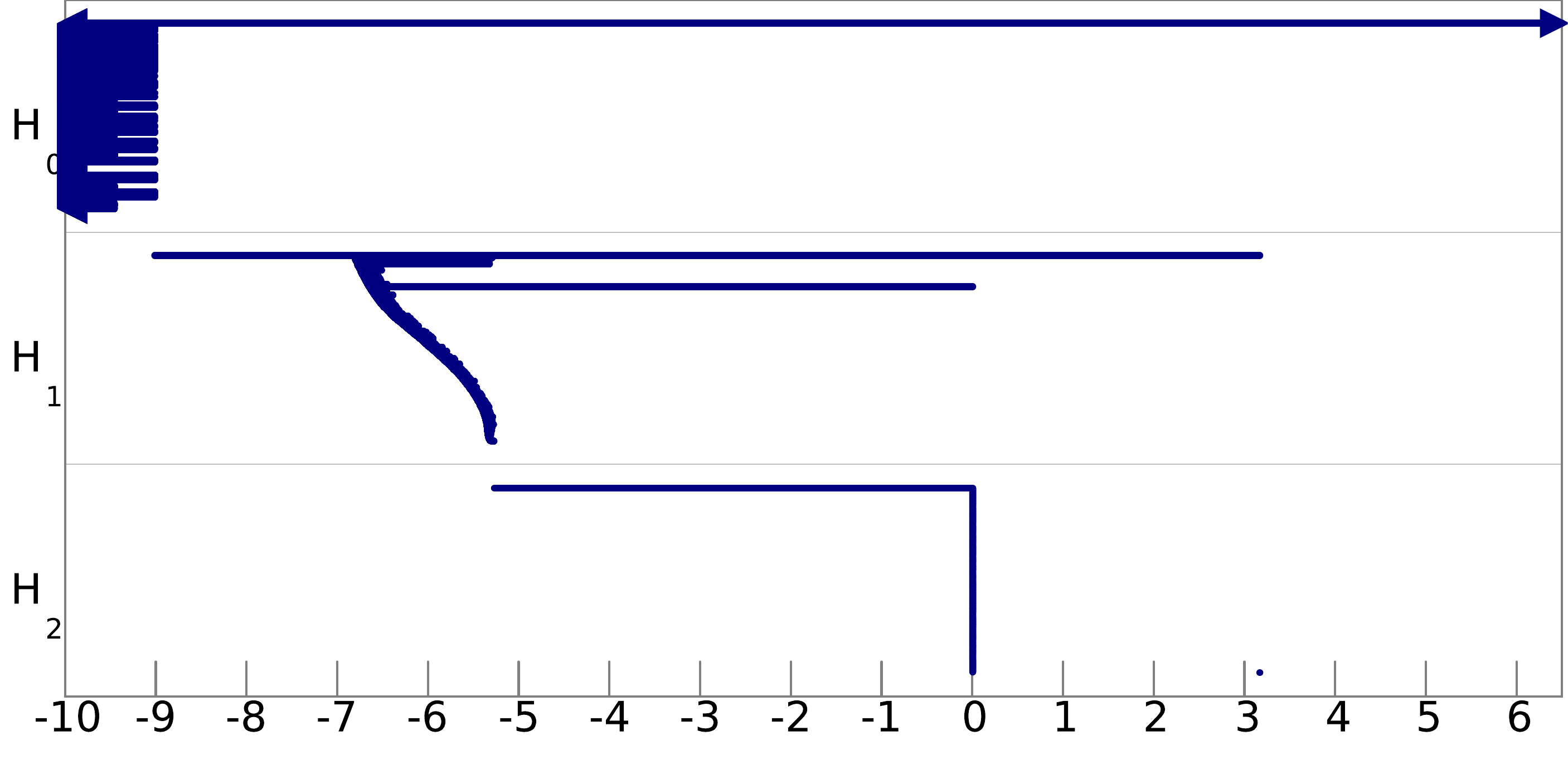